The focus of attention region (FOA) approach to object recognition is notable in part for its reliance on feature vectors capturing pattern information in FOA regions, and one of the most common techniques is based upon histograms of edge orientation. This assignment is going to demonstrate the value of orientation histograms in a two class classification problem. Specifically, distinguish between images of Big Ben in London and the Eiffel Tower in Paris.

Unlike the previous assignment, where a significant portion of the assignment was the work required to create your own novel approach, in this assignment you will be given strict guidelines with respect to what to compute and how to evaluate the features you are producing in terms of classifcation accuracy. Through following the recipe provided, you are likely to develop a detailed appreciation for orientation histogram and the Bhattacharyy coeficient as a basis for comparing histograms/images

The step laid out below for completing this assignment should be followed carefully and at no point should you be using library functionality for any of the steps. To put this another way, since the goal of the assignment is a detailed understanding of the steps involved, building the code is a part of this excercise.

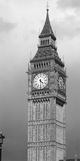
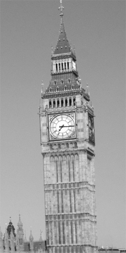
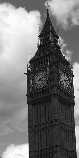
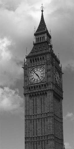
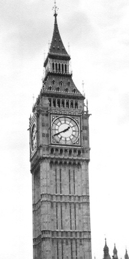
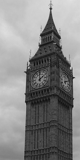
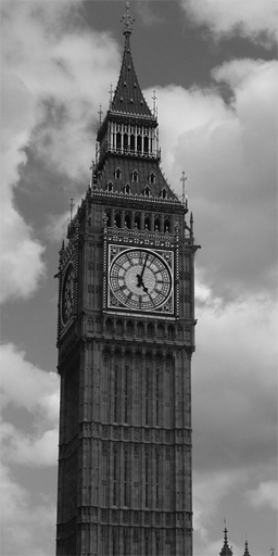
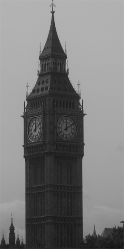
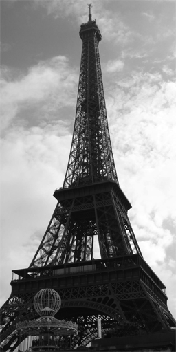
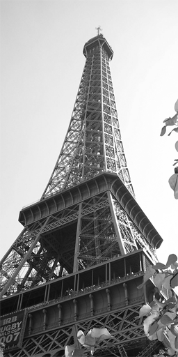
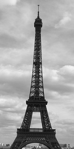
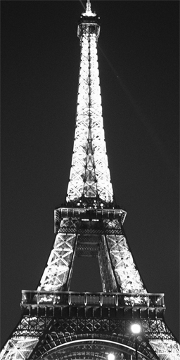
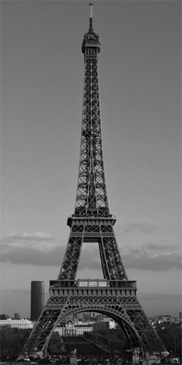
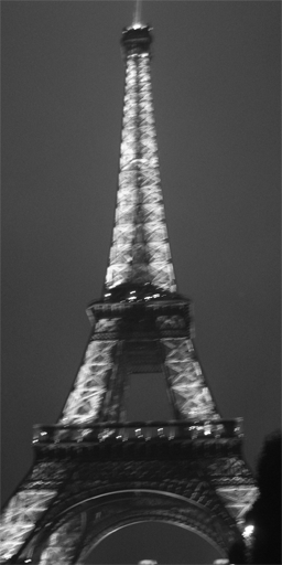
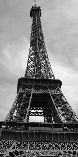
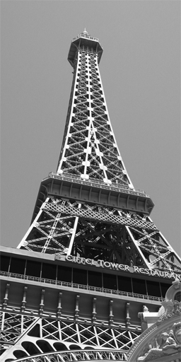
You are being provided eight images of Big Ben and eight images of the Eiffel Tower:

There is a imgs.zip zip file with all eight images. Note the images are in 256 by 512 pixels in size and are stored as color PNG images even though they've been converted to grayscale. This will simplify reading them in some systems.

You are going to create similarity matrices that compare all sixteen images and your going to do this first using image correlation as a baseline. Then you are going to analyze these similarity matrices using a two-fold cross validation protocol. Examples of the types of results you should expect are included here.

A note here, when you first read in your images, you are strongly encouraged to remap the pixel values for each image to the range 0 to 1. Doing so will make comparing what you get to whay is shown here much easier. That said, you are unlikely to ever see a perfect match of values or recognition rates. If what you get is close you are likely on the correct track.

First build a sixteen by sixteen similarity matrix where similarity is measured in terms of correlation between image pairs.

Here is an example:

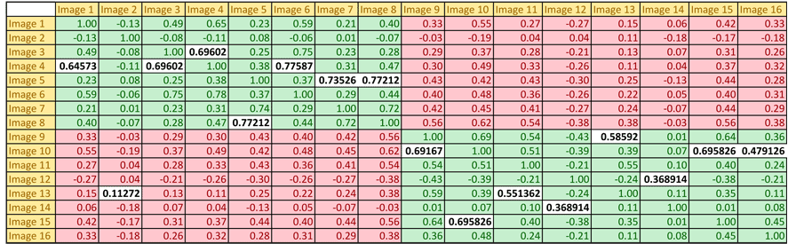
Note that the first eight images are Big Ben and the remaining eight are the Eiffel Tower. The green areas indicate comparisons between the same places and red comparisons between different places. Seen in this way, the correlation scores look very promising with the nearest neighbor of the same object in 15 out of 16 cases: notice the high correlation score per column is highlighted.

However, this simple analysis can be misleading. Consider instead what we see with a two-fold cross validation experiment using 10 randomly assigned splits of the data. The results are shown here:

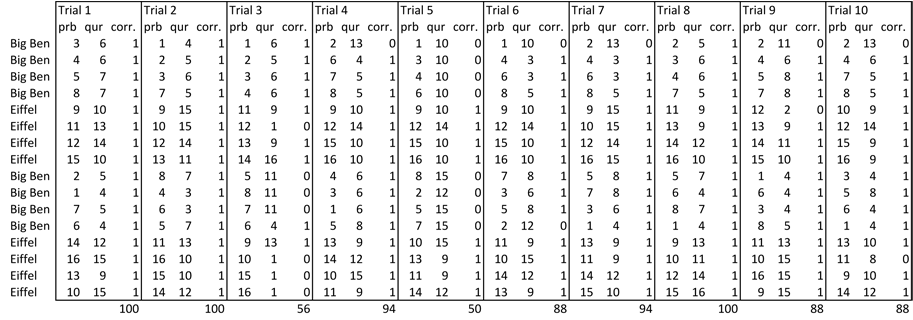
There are three columns for each of the ten random trials. In each trial, the images of each object are split randomly into two sets: training and testing. For a given row, the first column indicates a probe image drawn from the test set. It is compared against all training images and the closest training image is returned. This is shown in column two. Column three has a 1 iff the closest training image is of the same object.

Along the bottom the recognition rate is shown, and notice it ranges all the way from 50 percent to 100 percent. This is not so good, and motivates the heart of the current assignment.

For this assignment you are to implement a SIFT style feature vector that histograms gradient orientation in 16 small patches centered on an FOA point. To make this assignment simpler, the step of locating FOA points is replaced with a simple tyling strategy. Specifically, for each FOA position identify the 16 by 16 pixel square centered on the FOA point. Technically, shift down and left a half pixel to overcome issue that the center is not itself a pixel.

Now, divide the area into 16 (4 by 4) areas. Each of these will be 4 pixels on a side. For each of these, do a soft histogram of edge orientation by the following procedure. Divide the minus pi to pi range of orientations into 16 cells. For a given pixel, increment by a value of 2 the cell closest to its true orientation and 1 on either side. To build the feature vector for the entire FOA, concatenate the 16 histograms into a single 256 value feature vector.

Here is a detail that matters. Only have pixels vote for orientations in the histogram if their edge strength is above a threshold. For images with dynamic range normalized between 0 and 1, a threshold of 0.1 will serve nicely. Also, for consistency accross implementations, use the Sobel masks to measure edges.

Since you are not being asked to do the localization phase of an FOA procedure, instead, simply concatenate the feature vectors for a tiling of the 16 by 16 regions across the entire image. Hence, when you are done, you will have a single large feature vector representing each original image.

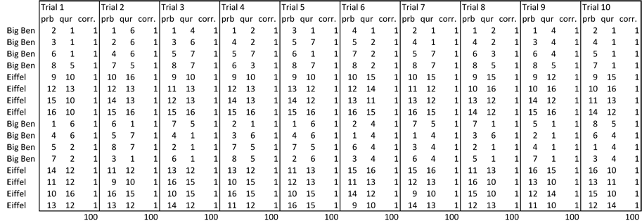
If you then compare images using the Bhattacharyy coeficient you should see two-fold cross validation recognition results similar to these:

Please submit a single zip or tar file through RamCT containing everything necessary to compile and run your program on a department unix workstation.

If you have special reasons for not using, or at least porting your code, to the department workstations please work with in advance to come up with alternate arrangements.

Ross Beveridge 4/23/2012